TL;DR
Spec plate · SGS on AMR Rosie- SGS is a tiny change to PPO. It keeps a fixed pool of task configurations and resamples resets toward the ones the policy solves about half the time. The authors' code isn't out yet, so we wrote it from the paper. Our kernel matches the per-configuration weight table on the project page exactly.
- At laptop scale it is the difference between learning and not learning. With 4,096 environments and 15.7M steps, SGS reached 0.602 held-out success on the standalone Rosie 1430 arm, against 0.164 for uniform sampling. On the 7-axis War Machine A/B cell it reached 0.512 against 0.041.
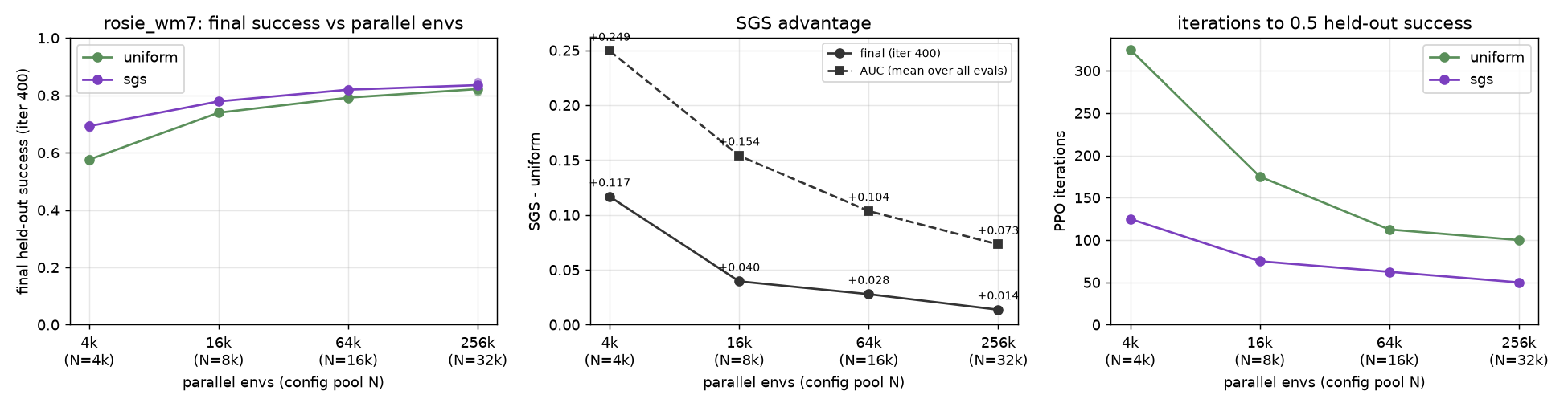
- At GPU scale it is a constant 2× speed-up, not a growing gap. From 4k to 262k environments on L40S GPUs, SGS reached 50% held-out success in half the PPO iterations at every scale. Its lead in final success shrank from +0.12 to +0.01, because both samplers approach a ceiling of about 0.8 on our task. This doesn't reproduce the paper's growing advantage with scale, and we think our task simply runs out of headroom.
- Demonstrations help as reset states, not as labels. Starting episodes along our own weld planner's paths taught the policy steep seams that SGS alone missed: 0.96 against 0.65 on held-out steep seams, with 3.6 mm seam tracking against 9.5 mm. Behaviour-cloning warm starts from the same 12 plans made every run worse.
| Setting | Parallel envs | SGS | Uniform | Takeaway |
|---|---|---|---|---|
| PointMaze toy (2D, 4 rooms) | 4,096 | 0.947 | 0.948 | Easy task: no difference |
| Rosie 1430 arm, 6 axes (laptop CPU) | 4,096 | 0.602 | 0.164 | 3.7× uniform |
| War Machine A/B cell, 7 axes (laptop CPU) | 4,096 | 0.512 | 0.041 | Uniform barely moves |
| War Machine A/B cell (L40S, 400 iters) | 4,096 | 0.692 | 0.576 | 0.5 in 125 vs 325 iters |
| War Machine A/B cell (L40S, 400 iters) | 262,144 | 0.835 | 0.822 | 0.5 in 50 vs 100 iters |
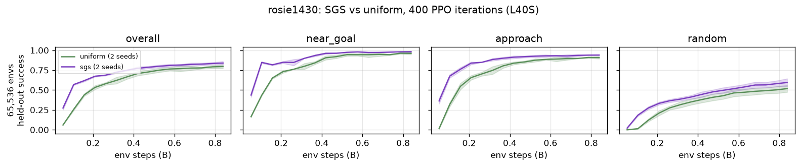
| Rosie 1430 arm (L40S, 400 iters) | 65,536 | 0.839 | 0.796 | 0.5 in 50 vs 100 iters |
| War Machine + planner path resets (steep seams held out) | 32,768 | 0.960 | 0.646* | *SGS without path resets |
A balanced data diet
Reset-based reinforcement learning has become a strong recipe for robot skills. Instead of asking a policy to stumble from a fixed start state into a sparse reward, you give it a large pool of starting states and goals, some of them already close to success. OmniReset [2] showed that diverse resets plus massively parallel simulation can learn dexterous manipulation without shaped rewards or demonstrations.
Zhang, Guaman Castro, Yin, Dagnino, Gupta, Scalise and Boots ask what happens when you push that recipe to harder tasks and far more parallel environments [1]. Their answer is that uniform sampling over the reset pool wastes a growing share of each batch. Most configurations are either already mastered (success near 1) or still out of reach (success near 0), and neither gives PPO a useful gradient. Adding environments just adds more of that waste.
Their fix is Success Guided Sampling (SGS). Before training, draw a fixed pool of N task configurations τ = (s0, g, e): start state, goal, environment variation. Keep the last H Boolean outcomes for each one, and estimate its success rate pi as their mean. At every reset, sample the next configuration from a Beta-shaped kernel that peaks at a target success rate t:
# Beta(1+κt, 1+κ(1−t)) shape, peaked at the target success rate t
w_i  = max( (p_i + ε)^(κ·t) · (1 − p_i + ε)^(κ·(1−t)) , ε )
ℓ_i  = log(w_i + ε)
P(i) = softmax(ℓ / T)          # temperature T = 2

# manipulation preset: t = 0.5,  κ = 1, ε = 1e-4, H = 100, N = 32,768
# locomotion preset:   t = 0.66, κ = 5, ε = 1e-8, H = 100, N = 104,000
That is the whole method. Rewards stay simple (a shared Boolean success term plus small regularisers), and PPO is unchanged. The paper trains with up to 220 (just over a million) parallel environments. At that scale it reports 70% success on a Franka nut-threading task where uniform sampling gets 6% and Prioritized Level Replay (PLR) [3] gets 5%. On multi-terrain quadruped locomotion it reports 73% against PLR's 54%. It also notes that on simpler insertion tasks SGS performs about the same as uniform sampling.
The kernel is gentle. Play with it below. With the manipulation preset, a configuration that has never been solved is still sampled at 14% of the peak rate, so the sampler never stops checking whether it has become learnable.
When we started, the authors' code was listed as "coming soon", so we implemented the sampler from the equations. That project-page table was the best independent check available. It confirmed we had read the exponents, the flooring at ε, and the temperature correctly. In a training loop the sampler sits between "episode ended" and "reset environment":
done = terminated | truncated
ids  = done.nonzero().squeeze(-1)
# record each finished episode's outcome against its config
sampler.update(env.config_ids[ids], success[ids])
# draw the next configs from the kernel
env.reset_envs(ids, sampler.sample(ids.numel()))
The history update is fully vectorised in PyTorch and handles many environments finishing the same configuration in one step. The same code runs on a laptop CPU and at a quarter of a million environments on a GPU.
A toy that is too easy
Our first testbed was a 2D point mass in an arena split into four rooms by walls with doorways. A configuration is a layout (one of eight), a start and a goal, and its difficulty is the number of doorways to cross. The reward is +10 for reaching the goal, with a tiny action penalty.
With 4,096 environments, a pool of 16k configurations and 250 PPO iterations (about 33M steps, 2 seeds), uniform sampling and SGS finished level: 0.948 and 0.947 held-out success. PLR collapsed to 0.392. It concentrated on a narrow set of configurations with large advantage estimates and generalised poorly.

This matches the paper's own observation that SGS performs comparably to uniform sampling on simpler tasks. The sampler statistics explain why. The 18% of configurations on the "frontier" (success between 0.1 and 0.9) received 31% of the resets: a real but modest tilt. When uniform sampling already learns, a gentle reweighting has nothing to fix. To see a difference we needed a task where uniform sampling struggles.
From a point mass to a welding arm
We build Rosie welding robots, so the natural next testbed was our own hardware. We used the robots' production descriptions: URDF kinematics and joint limits, the collision spheres used by our motion planner, and the planning rates. The task is the step every weld starts with: bring the torch to a seam at the right standoff and angle, from wherever the arm happens to be.
Our first environment modelled the War Machine cell, a Rosie arm working beside a two-station rotisserie positioner, as a 6-axis arm with the positioner frozen at zero and seams fixed in the world. SGS beat uniform clearly there (0.766 against 0.608, with PLR at 0.089).
Then the engineer who designed the cell pointed out that the cell description drives seven axes, and that the War Machine is an A/B cell whose tables turn the part during a weld. We had simplified away the positioner, the part of a welding cell that does most of the work. We froze the old environment as a legacy baseline, kept its numbers for reproducibility, and rebuilt both robots properly (§ 04). Lesson: read the description's own list of driven axes and its work frame before choosing a convenient subset.
What it took to make sparse reward learnable
The very first Rosie environment learned nothing at all: zero successes after 2.6M steps. Before tuning anything else we ran random-policy probes, measuring how often an untrained policy succeeds from each family of start states. That told us exactly what was wrong. Each fix below is a choice the paper also makes or motivates:
| Change | Why |
|---|---|
| Contact is a rigid stop with a small penalty, not episode termination | Near-goal starts sit 17 mm from the part. Random actions collided 57–84% of the time, ending the episode before it could succeed. |
| Tighter near-goal resets (0.02 rad of joint noise) | The paper's ablations agree: without useful near-goal resets, nothing learns. |
| Small initial policy noise, zero-initialised action head | A full-noise policy can't land a 10 mm / 5° window by chance. |
| Cartesian twist actions instead of joint velocities | Random near-goal success went from 5% to 16%. The paper credits operational-space control for the UR5e's results. |
| A 4,096-config pool instead of 16k at laptop scale | At ~1,300 episodes per iteration, a 16k pool leaves most histories at 0 or 1 outcome. The kernel down-weights both p = 0 and p = 1, so SGS can't find the frontier. |
The last row is the one most specific to SGS. A success-rate estimate needs visits. If the pool is so large that each configuration has been tried once, every estimate is 0 or 1 and the kernel has nothing to work with. At laptop scale we kept the pool roughly equal to the number of episodes in a few iterations. The rule we now follow for every new environment: measure random-policy success per start family before any long run; if the easiest family is not at a few percent, nothing will learn.
On the first (6-axis) Rosie environment, the sampler statistics show the mechanism directly. At iteration 20, 18% of configurations were on the frontier and received 58% of the resets. By iteration 60, 65% were on the frontier with 87% of the mass. By iteration 120, 68% were solved and the mass had moved on to the remaining hard ones.
Two weld cells, one task
Both environments share one parametrised implementation. The task in each:
- Configuration τ = (start joint angles, seam point, electrode direction), with the seam defined in the cell's work frame. The torch tip must end 17 mm back from the seam along the electrode, within 10 mm and 5°. Roll about the electrode is free, as it is in our planner.
- Goals lie on open faces of the part and the table, with the electrode tilted from the face normal. Every goal is checked reachable and collision-free by batched inverse kinematics before it enters the pool.
- Start families (OmniReset-style, and our difficulty axis):
near_goal(the IK solution plus 0.02 rad of noise),approach(+0.15 rad), andrandom(anywhere collision-free). - Actions are a tool twist (up to 0.25 m/s and 0.6 rad/s), mapped to joints with damped least squares and scaled into the robot's planning rates. Contact is a rigid stop. The reward is +10 on success plus tiny action penalties, over 100 steps at 10 Hz.
- Simulation is batched PyTorch kinematics: forward kinematics, Jacobians and sphere-versus-box collision for thousands of arms at once. MuJoCo, built from the same URDF, is used for rendering and to cross-check forward kinematics (they agree to within 10-5 m).
Rosie 1430: a standalone 6-axis arm
The first cell is the Rosie 1430 on a pedestal next to a welding table with a block-shaped part. Seams lie on the table top, the part top and the part's four side faces, with tilt up to 25°. The nozzle's collision spheres clear a face at 17 mm standoff only up to about 30°, so 25° keeps every goal feasible.
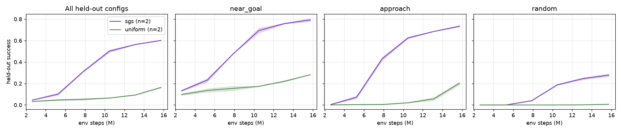
The random-policy probe gave 17.5% success from near-goal starts and 0% elsewhere, so no tuning was needed. SGS reached 0.602 against uniform's 0.164 (near-goal 0.793 vs 0.282, approach 0.734 vs 0.202, random 0.278 vs 0.007), and the seed ranges don't overlap. Uniform sampling stalls near its starting level for the first ~10M steps.
War Machine: an A/B cell with a moving work frame
The War Machine is the harder and more interesting cell. A Rosie arm (J1–J6) works beside an H-frame positioner that carries two rotisserie tables. One table is welded on while the operator loads the other. Planning uses either table, never both at once:
| Bay | H-frame (J9) | Driven axes | Held |
|---|---|---|---|
| A | 0 | J1–J6 + J7 (table A) | J8 = 0 |
| B | π | J1–J6 + J8 (table B) | J7 = 0 |
Three details made this cell faithful to how it is used, and each changed the environment design:
- Seams live in the moving work frame. They turn with the active table. The policy's 7-D action is a tool twist relative to the part, plus the table's rate. The arm solves a relative Jacobian (the tool's Jacobian minus the seam point's, for the table column), so a zero twist keeps the torch riding along with the turning part. This matches what our weld planner outputs: arm joints plus the active table, with the seam fixed in the table's frame.
- Downhand constraint. Success also requires the electrode within 25° of straight down, as in flat-position welding. Side and bottom faces can only be welded after the table turns them up, so the policy has to learn to use the positioner.
- Integration accuracy. A single Jacobian step per 0.1 s with the table at full rate drifted 2.32 mm per step on average. We now re-linearise five times per step (0.50 mm mean, 1.44 mm 95th percentile), at about 75% extra simulation cost.

Here uniform sampling barely leaves its starting level, and SGS is still climbing when the budget runs out. The probe gave 12–13% near-goal success per bay, enough for SGS to find a foothold and work outward. Uniform sampling spends most of its batch on approach and random starts it can't yet solve.
262,144 environments later
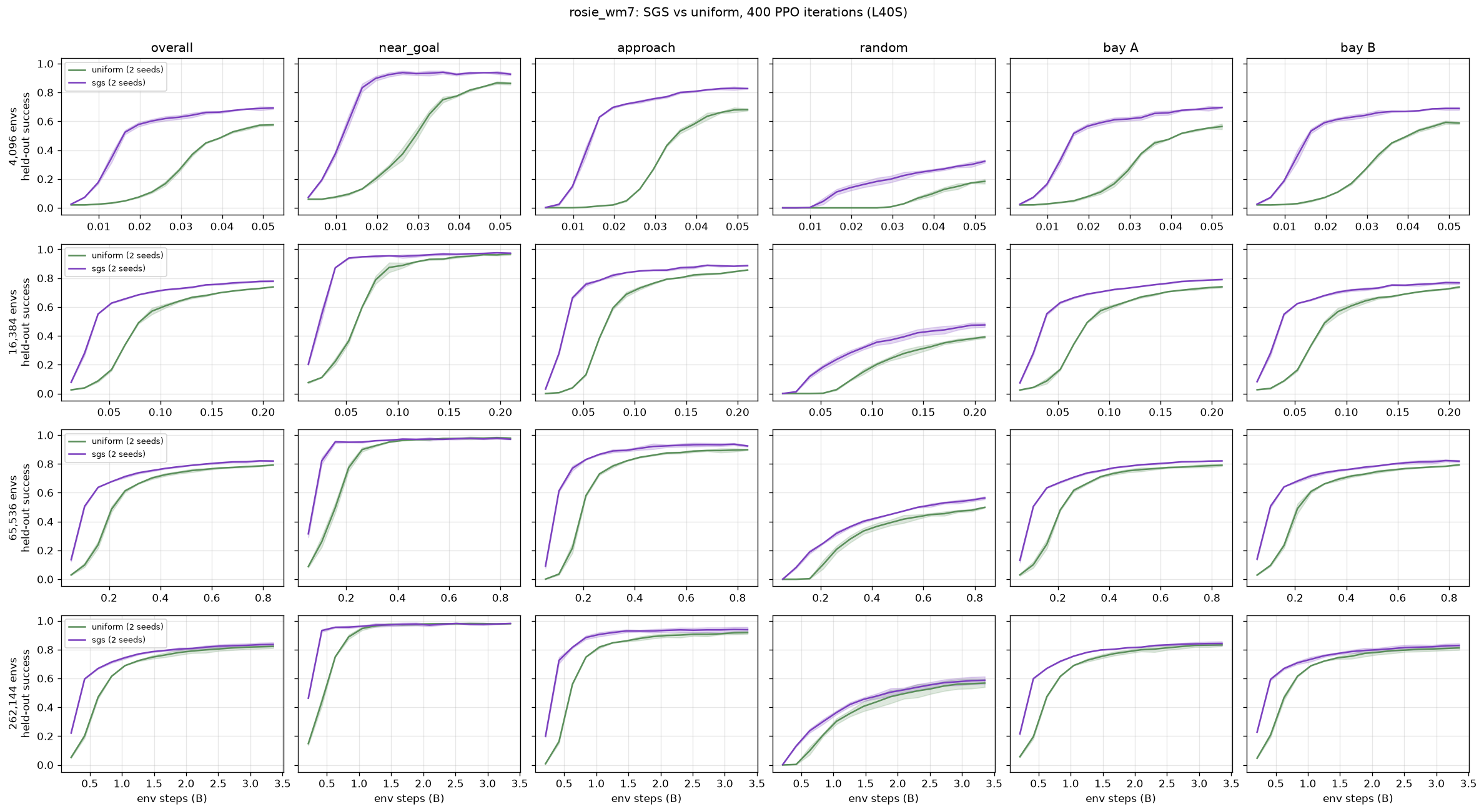
The paper's central claim is about scale: SGS's advantage should grow with the number of parallel environments, because uniform sampling wastes more of a bigger batch. The samplers, kinematics and environments are all PyTorch, so we moved them unchanged onto cloud L40S GPUs. As a check, a 4k-environment GPU run at iteration 125 matched the laptop baseline (SGS 0.524 vs uniform 0.048, against 0.512 vs 0.041 on CPU).
The sweep trained the War Machine task at 4k, 16k, 64k and 262k environments, plus the 1430 at 64k. Every run used 400 PPO iterations and 2 seeds per sampler, with evaluation on 2,048 held-out configurations. The pool grows with scale, as N = 4096·√(envs / 4096), reaching the paper's 32,768 at 262k environments. At the top end a run covered 3.4 billion environment steps in 54 minutes, about a million steps per second including evaluations. The whole sweep took 7.6 L40S-hours, about $17.
PPO iterations to 50% held-out success
Final held-out success (400 iterations)
| Envs | Pool N | Uniform | SGS | Iters to 0.5 | Iters to 0.7 |
|---|---|---|---|---|---|
| 4,096 | 4,096 | 0.576 | 0.692 | 325 → 125 | never → 375 (1 seed) |
| 16,384 | 8,192 | 0.739 | 0.779 | 175 → 75 | 325 → 188 |
| 65,536 | 16,384 | 0.792 | 0.820 | 112 → 62 | 188 → 125 |
| 262,144 | 32,768 | 0.822 | 0.835 | 100 → 50 | 150 → 100 |
| Rosie 1430 · 65,536 | 16,384 | 0.796 | 0.839 | 100 → 50 | 212 → 150 |
Two things are true at once. SGS is consistently faster: it reaches 50% held-out success in half the iterations at every scale, and 70% in a third to 40% fewer. But its final lead shrinks with scale, from +0.12 at 4k environments to +0.01 at 262k (within seed noise). The gap in area under the learning curve shrinks too, from +0.25 to +0.07. Here, more parallel environments mostly help uniform sampling catch up.
Why the paper's growing gap didn't appear
Both samplers converge to roughly 0.8, and the ceiling comes from the random-start family. At 262k environments, near-goal starts end at 0.98 and approach starts at 0.91–0.96 for both samplers, while random starts plateau between 0.54 and 0.61. At large scale our task stops being hard enough for uniform sampling to fail. With 262k environments, even an unfocused batch contains enough frontier configurations to learn from. The paper's large-scale wins come from tasks where uniform sampling collapses at every scale it tested (6% on nut-threading at a million environments), with contact-rich physics and long horizons. Ours is a kinematic reach with a 10 mm tolerance.
So we read this as "not tested properly yet" rather than "refuted". A fairer test of the scaling claim needs a task that still has headroom at 262k environments. That means a harder pool (more random starts, 1–2 mm tolerances, table motion during the weld), comparisons at fixed environment-step budgets rather than fixed iterations, more seeds, and contact physics. What did reproduce cleanly at every scale is the core mechanism: spending the batch on the frontier roughly halves the iterations needed to get competent.
Learning from our own weld planner
Rosie cells already have a GPU weld planner that produces collision-free approach, weld and retract trajectories for production programs. That raised an obvious question: can planner paths make the RL policy better? We tested the two standard ways to use demonstrations. The first is path resets: start episodes at states along planned approaches, OmniReset's "near goal along the path" idea. The second is a behaviour-cloning (BC) warm start.
The planner produced 18 dense plans for three sample parts, all in bay A. Turning them into training data taught us how the planner's output maps onto a policy's action space:
- Express plans as the policy would. The planner outputs arm joints plus the active table. Converted to a work-frame relative twist plus a table rate, and pushed back through the environment's own Jacobian integrator with substeps, the labels reconstruct the plan to 0.06 mm per step on average.
- Roll is free, but keep the planner's roll anyway. Success ignores roll about the electrode. Even so, labels that drop the planner's roll rate let the arm wander off the planner's joint path, with up to 41.7 mm open-loop error. Labels that keep it stay within 3.2 mm, and 856 of 856 perturbed replays reach the goal.
- Retime. Planner approaches run at only 10–18% of the joint rate limits: 182–510 control steps including a dwell, against a 100-step episode. We kept the collision-free geometric path and replayed it at 0.7 of the environment's limits, giving 27–80 steps.
- Respect real geometry. All 18 plans pass through our synthetic part box, because the real part occupies that space differently, so planner configurations turn the synthetic part off. 17 of 18 weld starts hold the torch 43–80° from vertical. Planner configurations therefore use the planner's own angle plus 5° as their downhand limit.
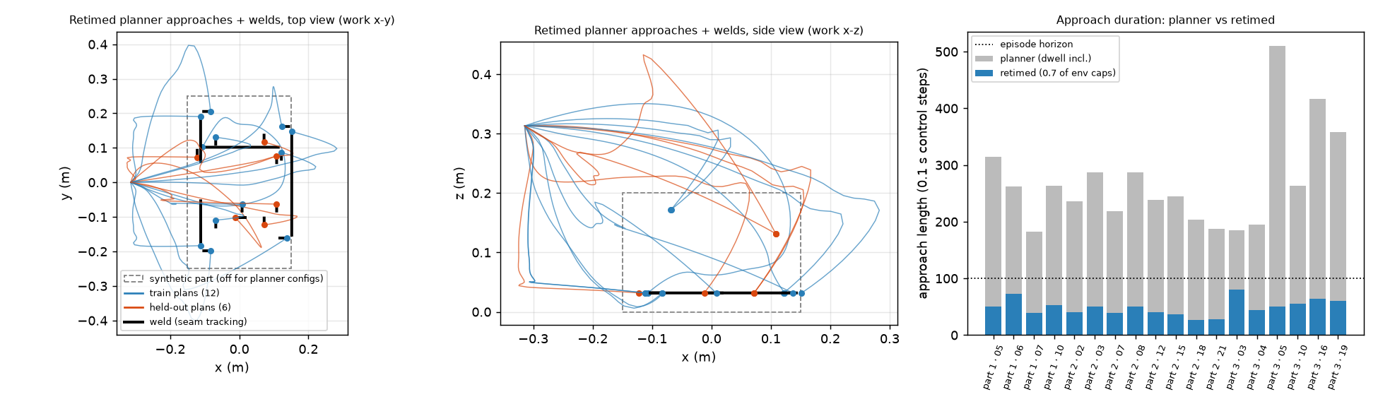
Every method used SGS, 32,768 environments, 160 iterations (168M steps) and 2 seeds. Plans were held out by plan, never by state. Split A holds out six plans with gentle seams (10–55° from vertical). Split B holds out three steep seams (67–74° from vertical) plus three others.
| Method | Standard pool | Held-out planner seams (A) | Seam tracking (A) | Held-out planner seams (B, steep) |
|---|---|---|---|---|
| (a) SGS from scratch | 0.723 | 0.917 | 9.5 mm | 0.646 |
| (b) SGS + 4,096 path-reset configs | 0.716 | 1.000 | 3.6 mm | 0.960 |
| (c) + BC warm start + BC loss term | 0.023 | 0.000 | 181 mm | — |
| (c1) BC warm start, no BC term | 0.028 | 0.000 | 158 mm | — |
| (c2) light BC with hindsight goals | 0.456 | 0.911 | 11.1 mm | — |
| (c3) BC loss term only (DAPG-style) | 0.677 | 1.000 | 4.4 mm | — |
Path resets: free gains where they matter
Path resets cost nothing on the standard pool (0.716 against 0.723, within seed noise) and fix exactly what SGS alone gets wrong. Trained from scratch, SGS never learns the steep planner seams where the torch sits 67–80° from vertical. With path resets every plan reaches 1.00. Split B shows that this transfers to unseen steep seams, with 0.960 held-out success against 0.646, even though the reset buffer held only two steep training plans, both from other parts. Seam tracking improves as well, from 9.5 to 3.6 mm.
Behaviour cloning: why it hurt
Every BC variant was worse than no BC. After 50 epochs of BC the policy's mean action on standard near-goal starts was 0.50, often saturated, against 0.001 for the zero-initialised policy. That destroyed the "barely move" prior that lets an untrained policy succeed from near-goal starts, which is precisely the foothold SGS bootstraps from. First-iteration training success fell from 14% to 4%, and the strongly cloned variants never recovered in 160 iterations. Hindsight goal relabelling didn't fix generalisation either. All 12 training approaches start from the same home pose and head to the same region, so a standard near-goal start is out of distribution for any labelling. With 12 plans, demonstrations are better used as places to start than as actions to copy.


The best policies
The best seeds from the scaling sweep, re-evaluated on a laptop CPU, reproduce their logged GPU scores exactly. The War Machine policy trained with 262k environments scores 85.0% held-out (near-goal 0.98, approach 0.96, random 0.61; bay A 0.86, bay B 0.84). The Rosie 1430 policy trained with 65k environments scores 86.0% (0.99, 0.95, 0.64). Every episode shown is a held-out configuration, so the policy never trained on these exact goals.
The films show successful episodes only, so read them next to those rates: the misses are mostly random starts, where about four in ten episodes time out. Everything plays at real time. The policy acts at 10 Hz and we interpolate joint angles to 30 fps.
Limitations and next steps
This is a faithful re-implementation of the sampler, not of the paper's experiments. The differences matter for interpreting our numbers:
- Kinematic simulation. There are no dynamics, drive model or contact physics; contact is a rigid stop, and accelerations are ignored. The paper uses full physics with contact-rich assembly.
- Loose tolerances. 10 mm and 5° is a reach, not a weld. Real welding needs 1–2 mm, which would make the task much harder and probably more favourable to SGS at scale.
- Simplified geometry. Fixtures and parts are boxes. The real parts behind the planner demonstrations are not in the collision model, so the planner's main skill, threading the torch around the part, is untested.
- Small sample. Two seeds per setting; the 262k-environment gap (+0.013) is inside seed noise. The planner data is 18 plans from one bay and three parts.
- Our own PPO. We use a small PPO implementation without the paper's asymmetric critic, and a fixed-pool PLR variant.
Next, in roughly this order: a harder pool with headroom at scale, compared at fixed environment-step budgets; a seam-tracking task with the table moving during the weld; part geometry in the collision model and more planner data, including bay B; a move to a physics simulator such as Isaac Lab or MuJoCo Warp; and a diff of our sampler against the authors' code once it is released.
How to reproduce
The code lives in the sgs-rl/ folder of advanced-metal-research/robot-policy-testing. That repository is private for now, because it vendors our robot descriptions alongside the experiment code. The sampler itself is a little over a hundred lines of PyTorch, and the equations in § 01 are enough to rebuild it. With access, the main experiments run with:
# set up (Python 3.12, uv) and run the test suite
cd sgs-rl && uv sync && uv run pytest -q

# random-policy probe per start family: do this before any long run
uv run python scripts/probe_random.py rosie_wm7

# one training run, then SGS vs uniform x 2 seeds side by side (~30 min on a laptop CPU)
uv run python -m sgs_rl.train --env rosie_wm7 --sampler sgs --num-configs 4096 --iters 120
ENV=rosie1430 SAMPLERS="uniform sgs" ./scripts/compare.sh 120 4096 0 1

# batch-evaluate a run and render MP4 + GIF + filmstrip
uv run python scripts/show_best_rosie.py --env rosie_wm7 <run_dir>
The GPU sweeps launch every sampler × seed × scale combination from a single entry point, one container per run. GPU runs are deterministic: re-running a configuration reproduces every per-plan outcome and the final score exactly.
References
- O. Zhang, M. Guaman Castro, P. Yin, I. Dagnino, A. Gupta, R. Scalise, B. Boots. A Balanced Data Diet: Addressing the Exploration Bottleneck in Mega-Scale RL for Robot Control. Conference on Robot Learning (CoRL), 2026. arXiv:2610.12465 · project page.
- P. Yin, T. Westenbroek, Z. Zhang, et al. Emergent Dexterity via Diverse Resets and Large-Scale Reinforcement Learning (OmniReset). International Conference on Learning Representations (ICLR), 2026. arXiv:2603.15789.
- M. Jiang, E. Grefenstette, T. Rocktäschel. Prioritized Level Replay. ICML, 2021. arXiv:2010.03934.
- J. Schulman, F. Wolski, P. Dhariwal, A. Radford, O. Klimov. Proximal Policy Optimization Algorithms. 2017. arXiv:1707.06347.
- M. Laskey, J. Lee, R. Fox, A. Dragan, K. Goldberg. DART: Noise Injection for Robust Imitation Learning. CoRL, 2017. arXiv:1703.09327.
- A. Rajeswaran, V. Kumar, A. Gupta, et al. Learning Complex Dexterous Manipulation with Deep Reinforcement Learning and Demonstrations (DAPG). RSS, 2018. arXiv:1709.10087.
- M. Andrychowicz, F. Wolski, A. Ray, et al. Hindsight Experience Replay. NeurIPS, 2017. arXiv:1707.01495.
- E. Todorov, T. Erez, Y. Tassa. MuJoCo: A physics engine for model-based control. IROS, 2012.
All figures, renders and videos on this page are our own, generated from our experiments. The paper's text and figures are not reproduced here; please read it via the links above.